Return is described as the motivating force and the principal reward in the investment process. It is a key method used by investors to compare alternative investments. Returns can be perceived differently by investors.
A typical investment’s return consists of two main components:
- Periodic cash receipts: This is the income component, such as interest or dividends.
- Change in the price: This is commonly known as capital gain or loss.
The term “yield” is often used in connection with the income component of return, relating it to some price for a security.
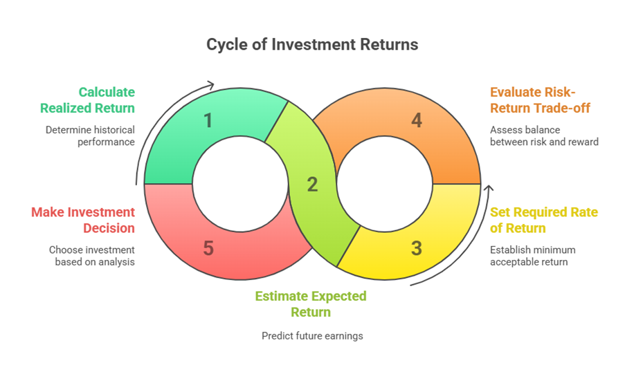
Returns can be classified based on when they are measured:
- Realised Return (Historical Return): This is the after-the-fact return that was earned or could have been earned.
- Expected Return: This is the return from an asset that investors anticipate they will earn over a future period. It may or may not actually occur.
The Required Rate of Return is the minimum rate of return that an investor expects to receive when investing in an asset over a specific period. This is also referred to as Opportunity Cost or Cost of Capital because it represents the highest expected return forgone from similar-risk investments available elsewhere. Sometimes, the required rate of return and expected return are used interchangeably.
Determining the acceptability of investment proposals often involves evaluating the trade-off between risks and returns. Risk-return analysis is used in decisions like capital budgeting, purchasing shares, and bonds.
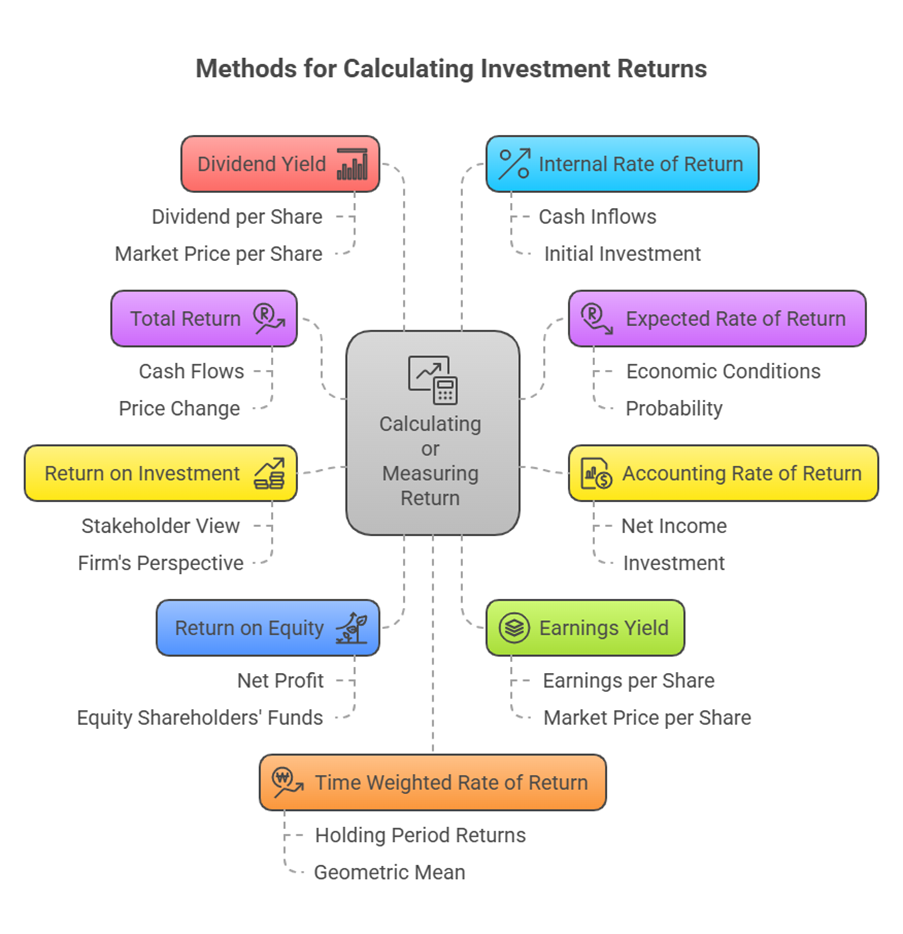
Calculating or Measuring Return
The sources present various methods for calculating or measuring return depending on the context and the type of information available.
1. Total Return
Total return measures the return for a specified period. It relates all cash flows received during a period to the amount invested. This return can be split into dividend and capital gains components.
Formula: Total Return = (Cash payments received + Price change over the period) / Purchase price of the asset
Expressed mathematically for one period: Total Return (%) = (D₁ + (P₁ – P₀)) / P₀ Where:
- P₀ = Initial price
- D₁ = Dividend in Period 1
- P₁ = Price at the end of Period 1
Example: If the current market price of a share is ₹600, and an investor buys 100 shares. After one year, they sell the shares at ₹720 and receive a dividend of ₹30 per share. Total Return (%) = (₹30 + (₹720 – ₹600)) / ₹600 = (₹30 + ₹120) / ₹600 = ₹150 / ₹600 = 0.25 or 25% [Calculated from source data]
Another example calculates “Holding period return” as: Holding period return = (90 + (900 – 950)) / 950 = 4.21%. Here, 90 is the cash payment (dividend) and (900-950) is the price change.
2. Expected Rate of Return
The expected return is the probability-weighted average of the possible returns.
Formula: E(R) = R₁ × P₁ + R₂ × P₂ + … + Rₚ × Pₚ Where:
- R = Rate of return
- P = Probability
Example:
| Economic Conditions | Rate of Return (%) (R) | Probability (P) | Expected Rate of Return (R × P) |
| Growth | 18.0 | 0.25 | 4.5 |
| Expansion | 11.0 | 0.25 | 2.75 |
| Stagnation | 1.0 | 0.25 | 0.25 |
| Decline | -5.0 | 0.25 | -1.25 |
| Total | 1.00 | 6.25 |
The expected rate of return is 6.25%.
Expected Return on Portfolio
The expected return of a portfolio is the weighted average of the expected returns of the assets it comprises.
Formula: E(Rp) = ∑ (wᵢ × E(Rᵢ)) Where:
- E(Rp) = Expected Return of the Portfolio
- wᵢ = Weight or proportion of the portfolio invested in security i
- E(Rᵢ) = Expected Return on security i
- n = Number of securities in the portfolio
Example: If 40% of funds are in share A (16% return) and 60% in share B (22% return). Expected portfolio return = (0.40 × 16%) + (0.60 × 22%) = 6.4% + 13.2% = 19.6%.
Another example with four securities:
| Security | Returns (per cent) (rᵢ) | Proportion of investment (xᵢ) |
| P | 11 | 0.3 |
| Q | 16 | 0.2 |
| R | 22 | 0.1 |
| S | 20 | 0.4 |
Expected return of portfolio = (0.3)(11) + (0.2)(16) + (0.1)(22) + (0.4)(20) = 3.3 + 3.2 + 2.2 + 8.0 = 16.7%.
3. Accounting Rate of Return (ARR)
This technique uses accounting information from financial statements to measure investment profitability.
Formula: ARR = Average annual net income / Investment Or ARR = Average annual net income / Average Investment
Example: If Average Profit after Tax is ₹40,000 and Initial Investment is ₹2,00,000. ARR = (₹40,000 / ₹2,00,000) × 100 = 20%. If using Average Investment, and assuming the investment depreciates to zero linearly over its life, Average Investment = (Initial Investment + Salvage Value) / 2. If Salvage Value is 0, Average Investment = Initial Investment / 2 [Based on example structure]. ARR = ₹40,000 / (₹2,00,000 / 2) × 100 = ₹40,000 / ₹1,00,000 × 100 = 40%.
4. Return on Investment (ROI)
ROI is a general term measuring overall return on various investment bases. It can refer to the return on equity funds, capital employed, or assets.
Formula: ROI = Return / Profit / Earnings × 100 / Investments
From a stakeholder’s view, a simple ROI can be calculated as (Sale Price – Initial Investment) / Initial Investment. From a firm’s perspective, investment might be total assets, net assets, or capital employed. ROI can be calculated from different bases like Total Assets, Net Assets, Shareholders’ Investment (Net Worth), or Capital Employed.
5. Return on Equity (ROE)
ROE indicates a firm’s profitability and potential growth.
Formula: ROE = (Net Profit after taxes – Preference dividend (if any)) / (Net Worth / Equity Shareholders’ Funds) × 100
6. Earnings Yield / EP Ratio
This ratio indicates the return on investment from the perspective of earnings generated per share.
Formula: Earnings Yield or EP Ratio = (Earnings per Share (EPS) / Market Price per Share (MPS)) × 100* *Also known as Earnings Price (EP) Ratio.
7. Dividend Yield
This measures the percentage return paid out as dividends relative to the share price.
Formula: Dividend Yield = (Dividend per Share (DPS) / Market Price per Share (MPS)) × 100
Significance: It helps investors know the effective return they will get from the dividend income on their investment at the current market price.
Example: If the market price is ₹25, paid-up value is ₹10, and dividend rate is 20% (on paid-up value, so ₹2 per share). Dividend Yield = (₹2 / ₹25) × 100 = 8%.
8. Internal Rate of Return (IRR) / Money Weighted Rate of Return (MWROR)
IRR is the discount rate that makes the Net Present Value (NPV) of all cash flows from an investment equal to zero. It’s the rate that equates the present value of cash inflows to the initial investment. MWROR is the same as IRR. It accounts for the timing and amount of cash flows.
Formula: Io = C₁/(1+K)¹ + C₂/(1+K)² + … + Cₙ/(1+K)ⁿ Where K = IRR. Alternatively, setting NPV to zero: NPV = C₁/(1+k)¹ + C₂/(1+k)² + … + Cₙ/(1+k)ⁿ – I₀ = 0 Where k = IRR, C = Cash flow, I₀ = Initial Investment, n = period.
Example (MWROR/IRR): Fund A has initial value ₹1,000 (Period 0). Cash flows received: ₹100 (End of Yr 1), ₹150 (End of Yr 2), ₹80 (End of Yr 3). Value at End of Yr 4 is ₹1,500. Equation: 1000(l+i)⁴ + 100(l+i)³ + 150(l+i)² + 80(l+i) = 1500. Solving for ‘i’ (IRR) yields approximately 3.46%.
9. Time Weighted Rate of Return (TWROR)
TWROR measures the rate of return earned per rupee invested over time, eliminating the effect of additional cash flows. It’s calculated as the geometric mean of holding period returns.
Formula: TWROR = [(1 + R₁) × (1 + R₂) × … × (1 + R<0xE2><0x82><0x99>)]¹<0xE2><0x81><0x84>ᵀ – 1 Where:
- T = Total number of periods
- R<0xE2><0x82><0x99> = Holding period return for period n
Example (using data from MWROR example): Holding Period Returns: Yr 0 to Yr 1: (1100 – 1000) / 1000 = 0.10 or 10% Yr 1 to Yr 2: (1200 – 1100 + 100) / 1100 = 200 / 1100 = 0.1818 or 18.18% -> Correction based on TWROR definition: Holding period return should be change in value excluding cash flows relative to start value. Source example calculation uses (1+i) = (1100/1000) * (1200/1200) * (1300/1350) * (1500/1380). The denominators (1200, 1350, 1380) seem to be values after cash flows. Assuming the TWROR calculation steps shown in the source: (1+i)¹ = 1100/1000 = 1.1 (1+i)² = 1200/1200 = 1.0 (This suggests a cash flow happened at the start of this period, adjusting the base value) (1+i)³ = 1300/1350 = 0.963 (1+i)⁴ = 1500/1380 = 1.087 Geometric Mean calculation shown: i = (1.1 × 1.0 × 0.963 × 1.087)¹<0xE2><0x81><0x84>⁴ – 1 = (1.1514)¹<0xE2><0x81><0x84>⁴ – 1 = 3.56%.
10. Return Calculation for Mutual Funds
Return on a mutual fund unit over a period can be calculated based on the change in Net Asset Value (NAV) and distributions.
Formula: rₜ = (NAVₜ – NAVₜ₋₁ + Iₜ + Gₜ) / NAVₜ₋₁ Where:
- rₜ = Return on the mutual fund for period t
- NAVₜ = Net asset value at time t
- NAVₜ₋₁ = Net asset value at time t-1
- Iₜ = Income at time t
- Gₜ = Capital gain distribution at time t
Alternatively: Total Return = (Distributions + Capital Appreciation) / NAV at the beginning of the period Where Distributions = Dividend Distribution or Capital Distribution Capital Appreciation = Closing NAV – Opening NAV.
Example: Beginning NAV = ₹50. During the year, ₹4 was distributed as income (dividend) and ₹3 as capital gains distribution. Ending NAV = ₹55. Total return = ((₹55 – ₹50) + ₹4 + ₹3) / ₹50 = (₹5 + ₹7) / ₹50 = ₹12 / ₹50 = 0.24 or 24%.
11. Risk-Adjusted Returns
These parameters evaluate the return of an investment (like a Mutual Fund) relative to the risk it assumed. Common measures include Sharpe Ratio and Treynor Ratio.
Sharpe Ratio: Measures Risk Premium per unit of Total Risk (Standard Deviation).
Formula: S = (Rᵢ – R<0xE2><0x82><0x99>) / σᵢ Where:
- Rᵢ = Return on Security/Portfolio
- R<0xE2><0x82><0x99> = Risk Free Rate of Return
- σᵢ = Standard Deviation of Return of Security/Portfolio
- S = Sharpe Ratio
Example: Index fund return = 11%, Treasury bills return (Risk-Free) = 6%, Standard deviation of index fund = 20%. Sharpe Ratio = (11% – 6%) / 20% = 5% / 20% = 0.25 [Calculated from source data].
Higher Sharpe Ratio is generally preferred.
Treynor Ratio: Measures Risk Premium per unit of Systematic Risk (Beta).
Formula: T = (R<0xE2><0x82><0x99> – R<0xE2><0x82><0x99>) / β<0xE2><0x82><0x99> Where:
- R<0xE2><0x82><0x99> = Average return of the portfolio (or return of security/portfolio)
- R<0xE2><0x82><0x99> = Average risk-free rate of return (or risk-free rate)
- β<0xE2><0x82><0x99> = Beta of the portfolio (or Beta of Security S or Beta of Fund)
Example: Portfolio return = 40%, Portfolio beta = 1.2. Market return = 25%, Risk-free rate = 8%. Treynor Ratio = (40% – 8%) / 1.2 = 32% / 1.2 = 26.67% [Calculated from source data]. Market Treynor Ratio = (25% – 8%) / 1.0 = 17% [Calculated from source data, market beta is 1.0]. Comparing the portfolio return with market return using Treynor’s measure shows the portfolio had a higher return per unit of systematic risk (26.67% vs 17%) [Based on example comparison context].
Other relevant mentions of return concepts include:
- Net Profit Ratio: Net Profit after taxes / Net Sales × 100.
- EBIT / Sales Ratio: EBIT / Sales × 100.
- Gross Profit Ratio: Gross Profit / Net Sales × 100.
- Operating Profit Ratio: Operating Profit / Net Sales × 100.
- Cost of Goods Sold Ratio: Cost of Goods Sold / Net Sales × 100.
- Operating Expenses Ratio: Operating Expenses / Net Sales × 100.
- Yield to Maturity (YTM): Discount rate that equates the present value of a bond’s future cash flows (interest payments and par value) to its current market price. An approximate formula is provided.
- Required Return on Incremental Investments: Calculated for decisions involving credit policy, considering total cost, collection period, and required rate of return. Formula: (Total Cost × Collection period / 360 or 365) × Rate of Return / 100.
In summary, the sources define return as a reward for investment, comprising income and price changes. They distinguish between realized and expected returns and introduce the concept of a required rate of return. Numerous formulas and examples are provided for calculating various types of return, from simple total return and accounting ratios like ROI and ROE, to time-value-based measures like IRR (MWROR) and TWROR, and risk-adjusted metrics such as Sharpe and Treynor ratios, reflecting the diverse applications of return analysis in financial management.